The Dominance of Ones: A Handy Quirk of Numbers

Lead digit analysis
There are a lot of open datasets out there. I surfed around on the government's open data site0 and picked one mostly randomly. It's a count of the number of border crossings there were for different periods, broken down by port of entry and by category, like "trains", "trucks", "bus passengers", and "pedestrians."0 Here's what the raw data looks like:
| Port | Date | Measure | Value |
|---|---|---|---|
| Roma, Texas | May 2017 | Trucks | 760 |
| Roma, Texas | May 2012 | Trains | 0 |
| Piegan, Montana | Mar 2020 | Trucks | 168 |
| Roma, Texas | Dec 2021 | Bus Passengers | 128 |
| Roma, Texas | Mar 2021 | Trucks | 2661 |
| Roma, Texas | Aug 2021 | Buses | 14 |
| Westhope, North Dakota | Jul 2023 | Trucks | 105 |
| Warroad, Minnesota | Jun 2022 | Trucks | 401 |
| Richford, Vermont | May 2021 | Train Passengers | 24 |
| Sasabe, Arizona | Mar 2023 | Pedestrians | 45 |
| ... |
Let's look at the first digit of each of those counts. See that "760" for the first count? The lead digit is "7". Here's the lead digit for each of the above counts:
| Border Crossings Count | Lead Digit |
|---|---|
| 760 | 7 |
| 0 | 0 |
| 168 | 1 |
| 128 | 1 |
| 2661 | 2 |
| 14 | 1 |
| 105 | 1 |
| 401 | 4 |
| 24 | 2 |
| 45 | 4 |
| ... |
Now, think about the whole dataset. This one has 38,549 entries. Each of those entries has a lead digit. Let's filter out the "0" counts and ignore those. What percentage of those entries would you expect to have "1" for a lead digit?
There are nine possible digits if we exclude "0" as an option. So, would you think "1" would occur as the lead digit about one-ninth of the time?
I would imagine that if we were to count all the measurements where the first digit was "1" and then count all the measurements where the first digit is "2" and so on, we would find about the same number of "1"s and "5"s. After all, this data is as random as it gets. So, shouldn't the lead digit should be essentially random? Let's confirm that assumption.
I made a Python notebook that you can run yourself that counts the number of measurements in the border-crossing dataset that start with "1" and with "2" and so on. Here's the distribution:
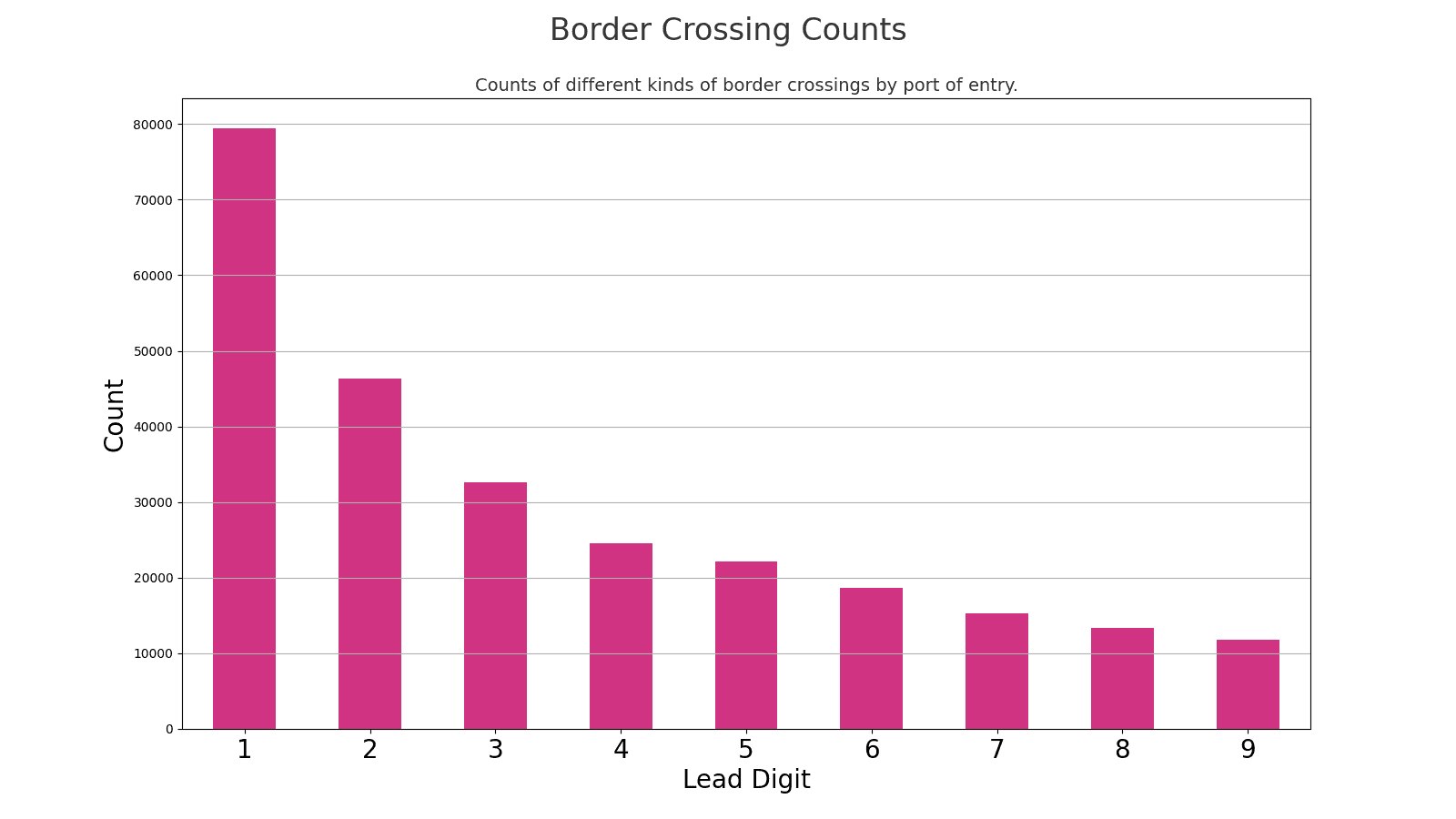
Well... Okay, that's weird.
There are a lot more "1"s. Shouldn't they all be even? Shouldn't there be as many counts starting with a "5" as a "1"? What's going on?
Benford's Law: Expect a lot of ones as leading digits in some data
This phenomenon is known as Benford's Law and is more common than you might think. Benford's Law states that the first digit is more likely to be lower than higher in many naturally occurring datasets. Specifically, "1" appears as the first digit about 30% of the time, while "9" appears as the first digit only about 5%.
It's a pattern that emerges naturally in a wide range of data. From financial records to geographical data, Benford's Law often holds. Here are some other datasets that I found on Data.gov where you can easily see it:
Here's the lead-digit breakdown from about a million real estate sale prices:0
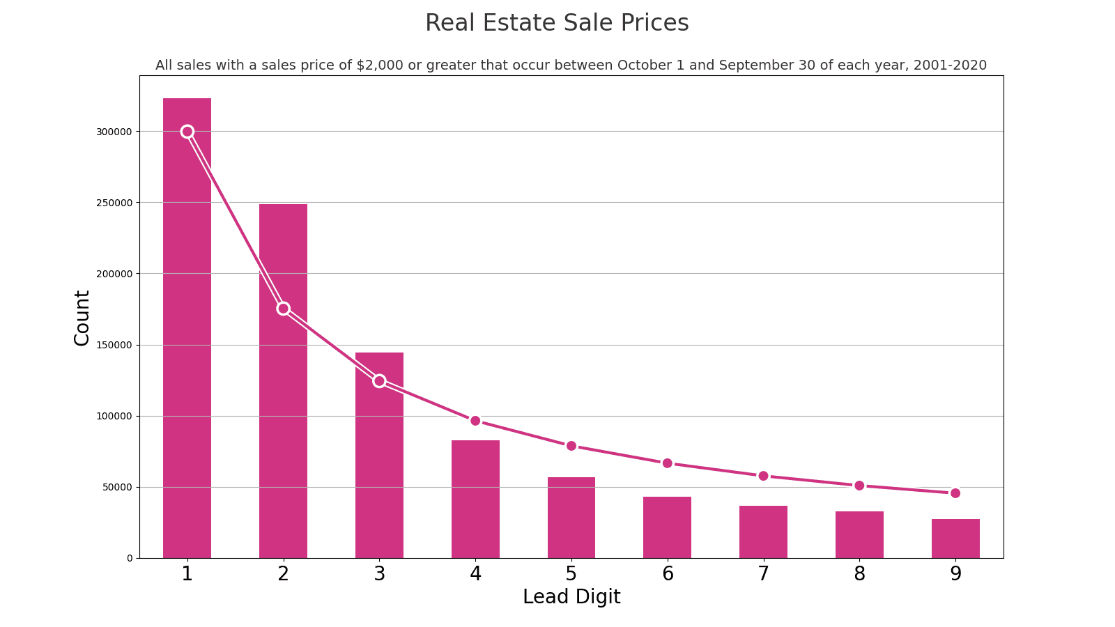
The dots superimposed over the bars show the proportions predicted by Benford's Law. They don't match exactly, but they do fit the overall pattern.
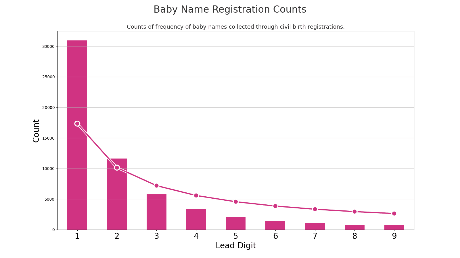
Here's a list of baby names, ranked by popularity, based on civil birth registrations.0 Each name has a count: How many registrations were there for each name?
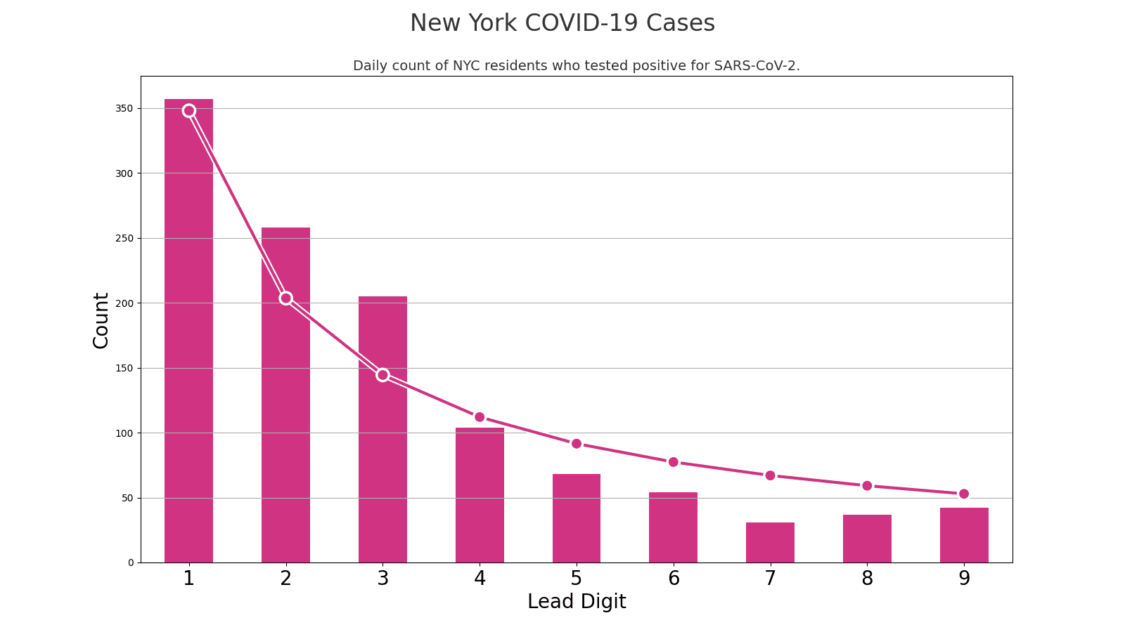
We all remember the daily counts of COVID-19 cases. Here's the lead-digit breakdown on the daily New York City case counts:0
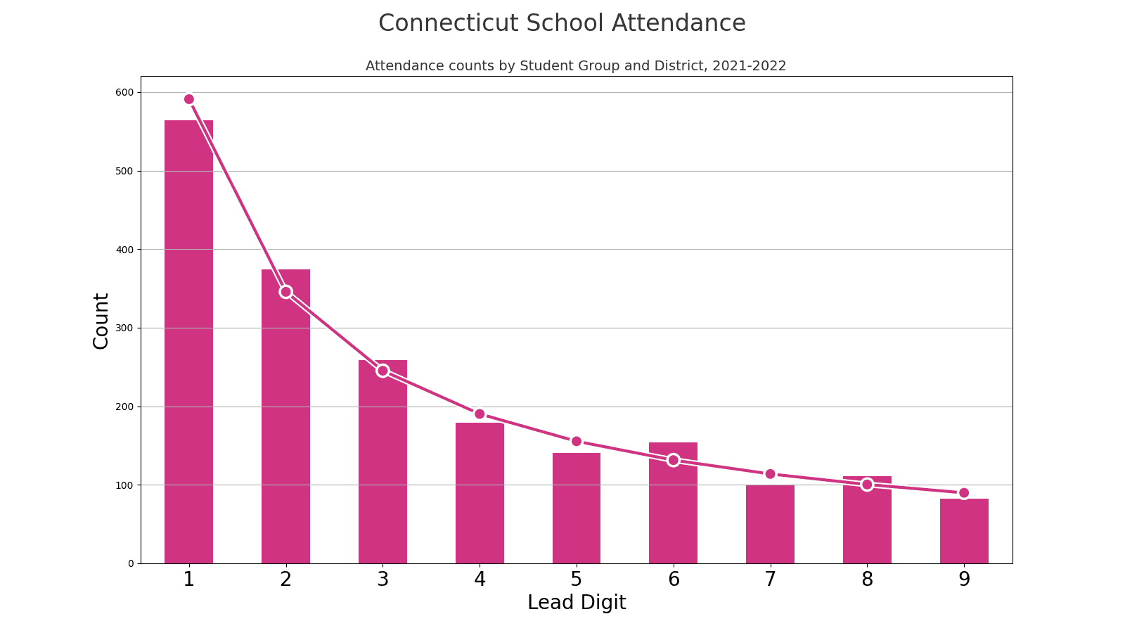
And here's the lead-digit breakdown from a bunch of different school attendance counts:0
An astronomer makes a discovery. About numbers.
Back in 1881, when the closest thing to a pocket calculator was a quick-witted accountant with a pencil, Simon Newcomb, an astronomer by trade, made a discovery that had nothing to do with stars but everything to do with digits.0 Newcomb's lightbulb moment didn't strike while stargazing or deep in complex calculations. Instead, it happened as he leafed through a well-thumbed logarithmic table book. In the days before digital convenience, these tables were the bread and butter of calculation, sort of like an ancient Excel spreadsheet but without the fun of accidental cell misformatting.
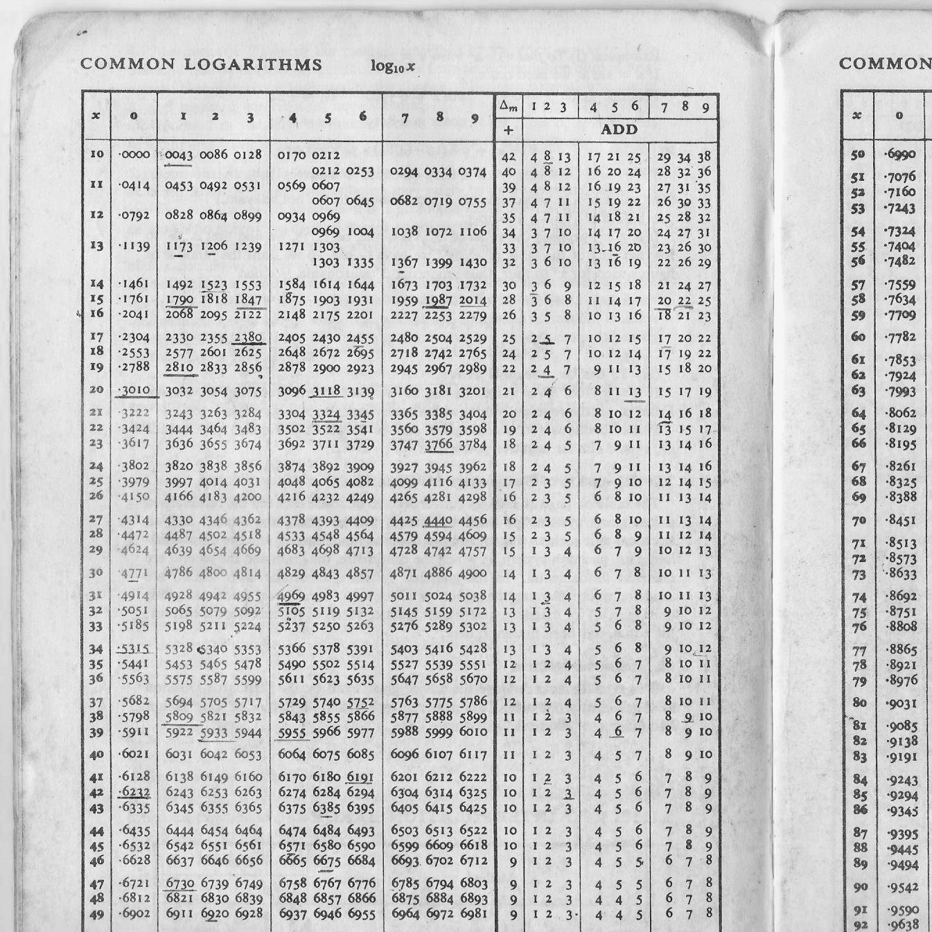
What caught Newcomb's eye was the curious case of the weary pages. The early sections of the logarithm book, the pages with numbers starting with '1', showed signs of significant wear and tear. It was as if these pages had run a marathon, while the latter pages looked barely out of the starting blocks. This wasn't just a case of page discrimination; it hinted at a numerical pattern. Newcomb theorized that numbers starting with '1' were not just the wallflowers of the numerical dance but were, in fact, the belle of the ball, getting picked far more often than their higher-digit counterparts.
Forming his hypothesis from this observation, Newcomb proposed that the first significant digit in many datasets is more likely to be '1' than any other number, with the chances diminishing as you count up to '9'.
It wasn't until 1938 that the idea gained widespread recognition, thanks to physicist Frank Benford. Benford expanded on Newcomb's observation, conducting a more thorough and extensive study covering a diverse range of datasets. He demonstrated that the first-digit distribution he observed closely matched Newcomb's earlier findings. Despite Newcomb's precedence, the law became known as Benford's Law due to his role in popularizing and formally documenting the phenomenon.
Okay, "some data"?
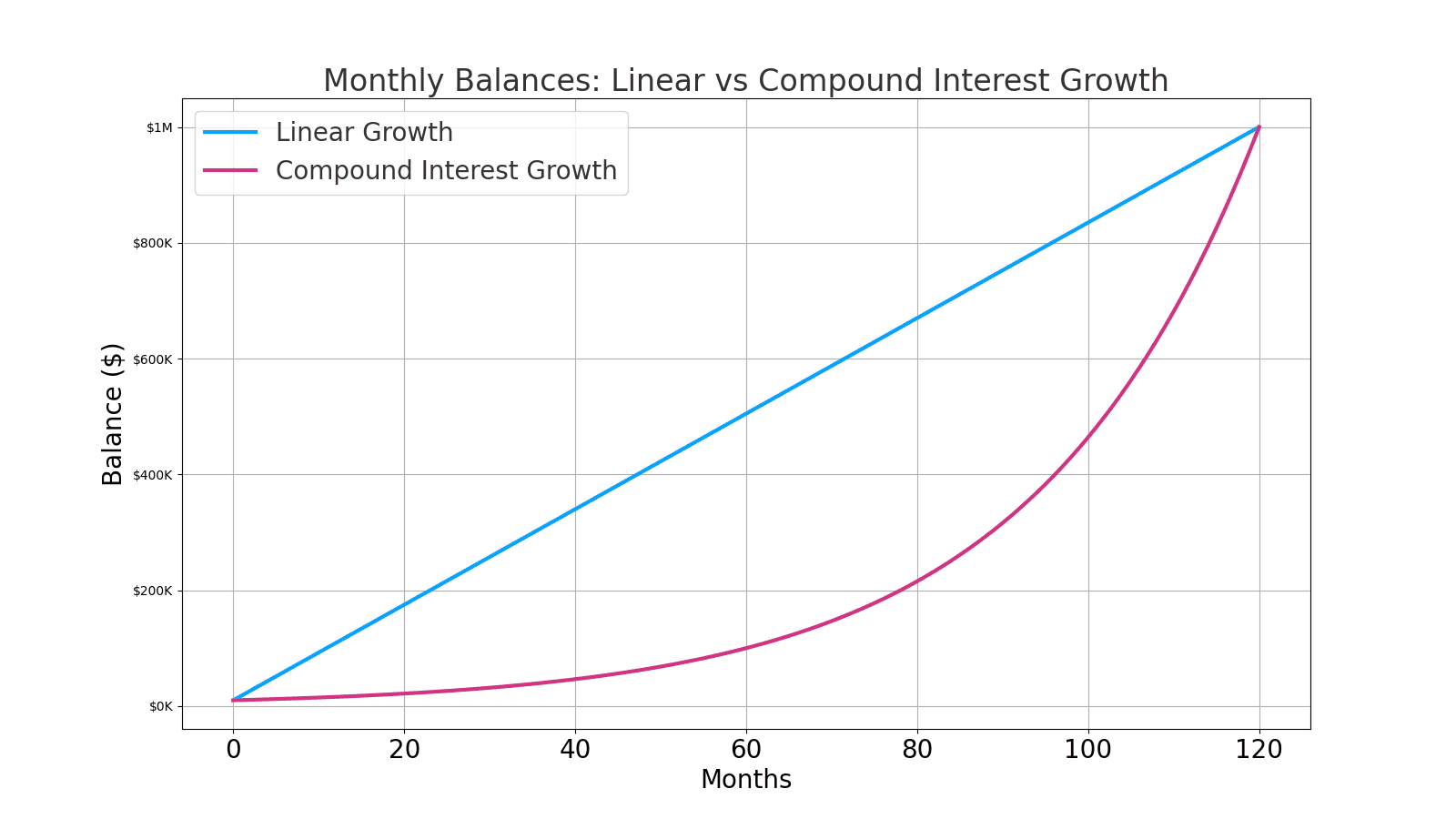
Let's look at a dataset where it doesn't happen. Here are two charts of two different bank account balances. Both grew over ten years from a principal of $10,000 to a final amount of $1,000,000. One of them grew as a result of compounded interest on the principal. The other grew in simple linear steps each month, ending up at the same point.
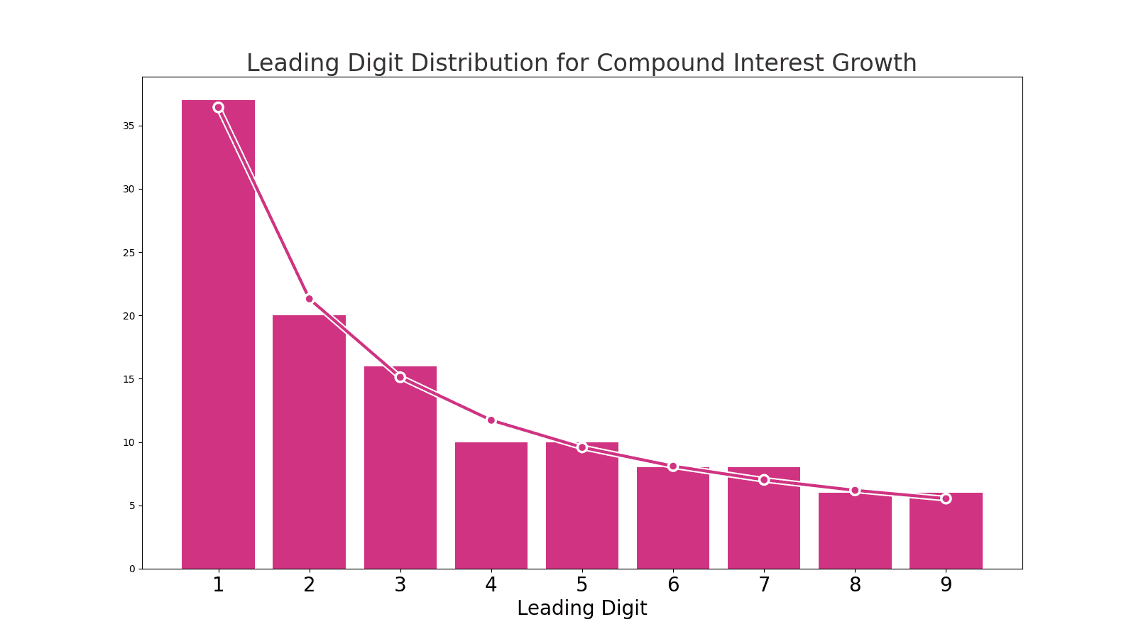
Suppose we do the same kind of analysis where we look at the breakdown of the first digits of the monthly bank balances in both accounts. In that case, we see Benford's Law reflected in the distribution of the compound interest, like in the natural datasets that we saw:
But, look at the lead-digit distribution for the bank account balances in the account that grew linearly over time:
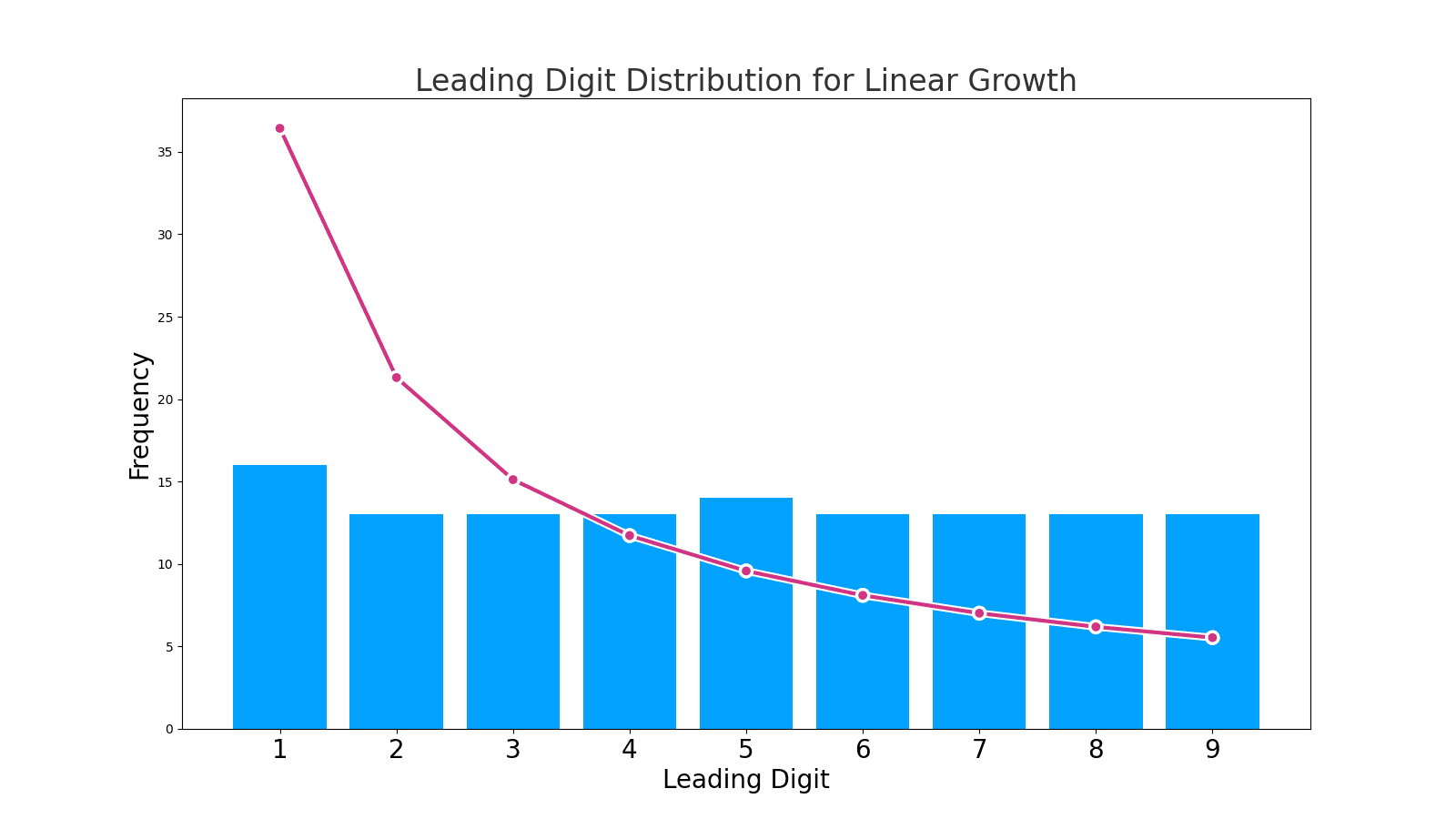
One kind of growth rate shows the distribution described by Benford's Law, and the other doesn't. Something that exponentially grows like an investment will show that kind of distribution. Someone regularly transferring money looks different.
Well, gosh, that sounds useful.
Applications
For example, money launderers trying to move money from one point to another without being detected will send money below specific amounts that trigger extra scrutiny. A typical scenario might be a money launderer with $35,000 to transfer who wants to avoid a $10,000 limit that will trigger additional reporting. They might break up their transactions into smaller chunks, like $9,500, $9,000, $8,500, and $8,000. Benford's Law can spot that in the deposit records if you have enough data and it's happening often enough.
In other words, money laundering looks different than legitimate transactions. It's like the numbers come with a built-in lie detector. Handy!
Let's simulate money laundering!
Imagine that you're a financial regulator, and you're monitoring two banks. You only have access to the total deposit amount for each day from each bank. There are a thousand deposits daily at each bank that are below the $10,000 reporting threshold, but someone is slipping structured transactions through one of the banks. Your job is to figure out which bank.
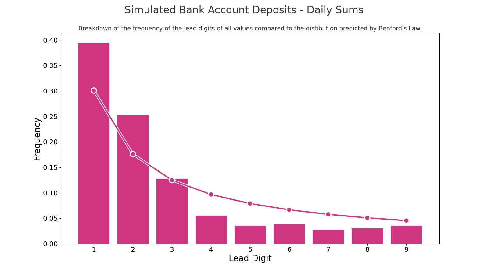
I made a Python notebook that simulates that. It randomly generates a thousand transactions for each of 365 days, and then it adds up the transactions for each day. We get a list that contains the total sums of deposits for each of the 365 days. Here's the lead digit breakdown for that list of simulated daily deposit totals:
Now, we simulate a second scenario: One where someone makes structured deposits. In the second scenario, we replace 1% of the natural transaction amounts with simulated structured transaction amounts. Our simulation is simple: They all randomly range from $9,500 to $9,999. We get another 365 daily sums, and here's the lead digit breakdown for that scenario:
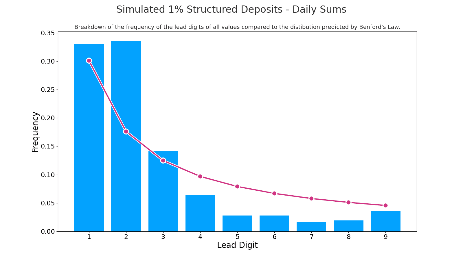
Does one of those distributions look "closer" to the distribution predicted by Benford's Law? Well, I don't know, they look about the same to me. Is there some way to measure it?
Yes! Financial forensics commonly uses a few ways to measure the differences. There's also one used a lot in AI.
Chi-Square Test
The Chi-Square test is a measure used to determine how well an observed distribution of data fits an expected distribution.0 In our case, we use it to compare the distribution of the first digits of our transaction data against the expected Benford's Law distribution. We expect this number to be higher if the distribution varies more from the distribution predicted by Benford's Law. Let's look at this statistic for both the simulated 'natural' transactions and the scenario with structured transactions buried inside:
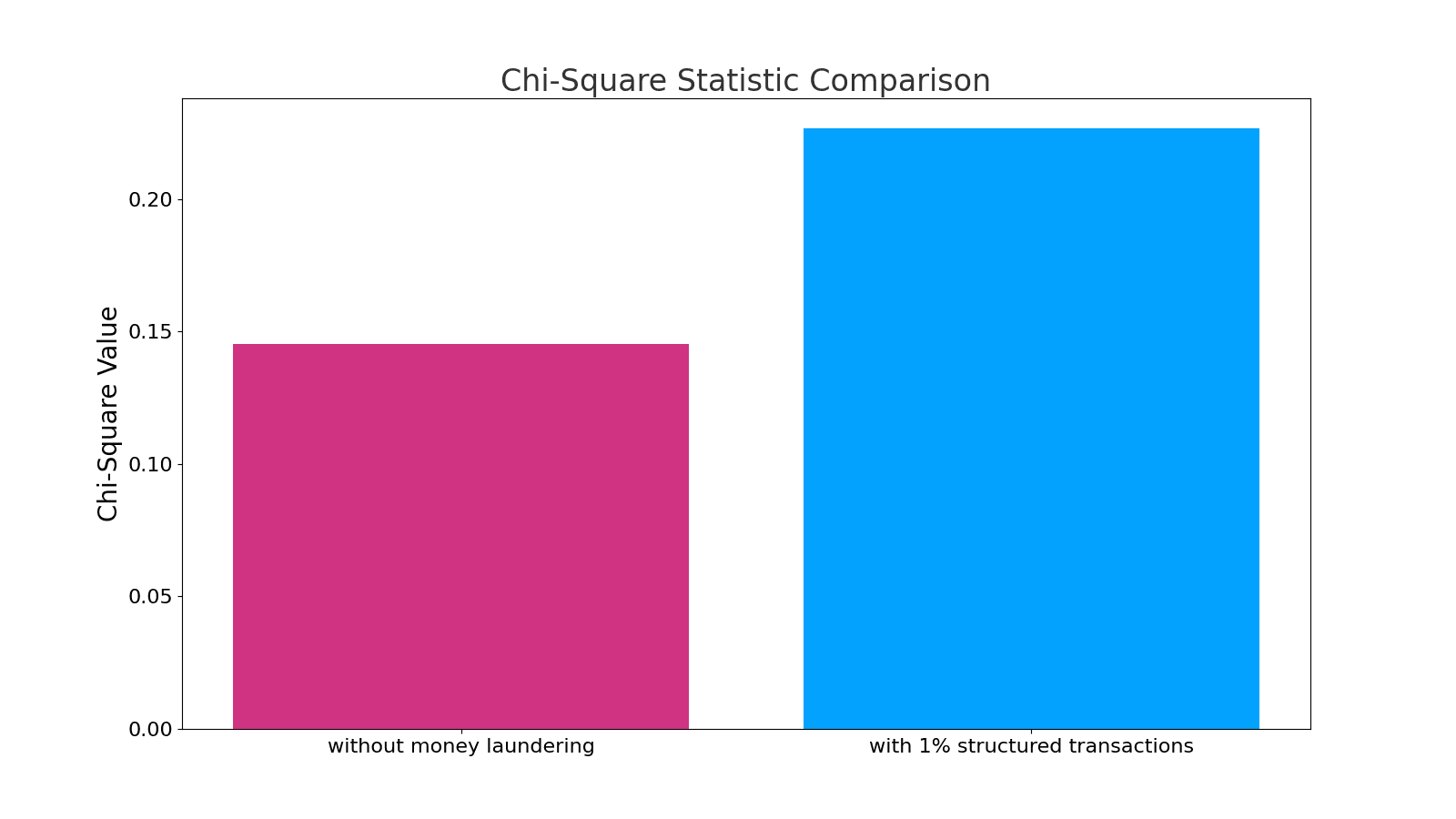
Wow, neat. It is higher for the structured transactions.
We can see which bank has money launderers for customers! They might not even know, but we can see it just by looking at the daily sums of deposits, without seeing the individual transactions. How cool!
Kolmogorov-Smirnov (KS) Test
The Kolmogorov-Smirnov (KS) test is another metric that measures the difference between two distributions.0 Here's how the two scenarios compare:
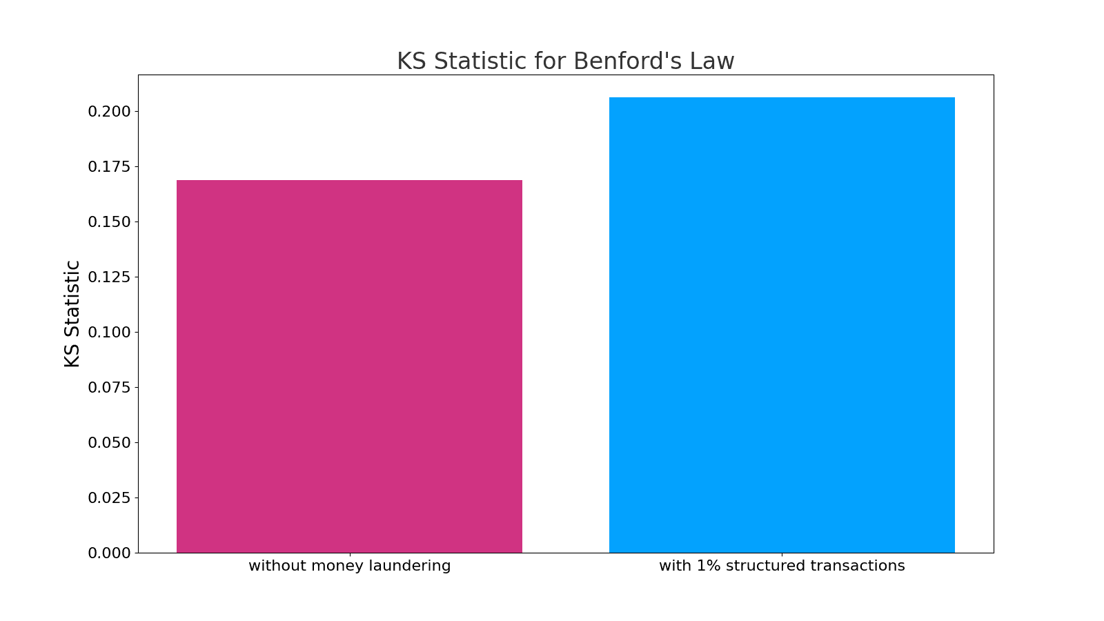
That one also shows the money launderers varying significantly from the normal transactions!
Kullback-Leibler (KL) Divergence
Kullback-Leibler is a loss measure that is used a lot in AI for things like RLHF evaluation,0 so why not...
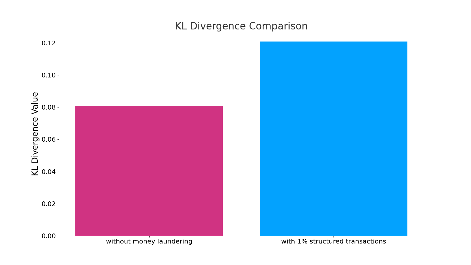
Cool, right? For all three measures, the scenario where just 1% of the transactions buried within an aggregate sum scored higher than the simulated natural number dataset. We can see that someone buried structured transactions in the data without seeing the individual transactions, only the daily summaries.
Real-world example: Crypto fraud by FTX and Binance
A Forbes investigation recently produced evidence of wash-trading aimed at inflating the market price of Binance's BNB token. One of the things that led them to the conclusion that FTX and Binance colluded to manipulate the crypto markets was, "there appears to be a lack of randomness to these flows that would likely be apparent if they were rooted market related economic activity."0 And we know exactly what that sentence is talking about: The amounts on the transactions didn't correspond with the distribution predicted by Benford's Law.
Other applications
Catching financial fraudsters is cool, but there are lots of other applications. You can use Benford's Law to detect the JPEG quality setting that was used to encode an image, for example. Using the JPEG coefficients from the luminance channel of already compressed JPEG images, and without using any machine learning, an algorithm can predict the quality setting used to encode the image nearly 90% of the time.0
AI applications
AI is all about statistics, so it's relevant that there's a quirk of statistics where natural data looks different from fake data.
Data for training AI models is increasingly critical, and much of it lately is fake. We use AI to generate training data for AI models because we don't want to feed real personally-identifying information and real financial data into the models. So, we make up fake names and fake numbers when necessary. The training data needs to be realistic.

The researchers trained image-recognition models using training sets of handwritten numbers that were truly random, and others that expressed the distribution predicted by Benford's Law. As hypothesized, the models trained on numbers where lower digits were more common lead digits were better at recognizing handwritten financial figures than the models trained on random handwritten numbers.0 Conversely, when the numbers were not financial figures, the models trained numbers with lower lead digits performed worse than the models trained on truly random strings of digits.
You can also apply Benford's Law to detecting AI-generated content. Researchers have explored using Benford's Law to detect GAN-generated images, which are often used to create deepfakes. By analyzing the distribution of the most significant digit for quantized Discrete Cosine Transform (DCT) coefficients, researchers can extract a compact feature vector from an image. If the distribution of these features deviates significantly from Benford's Law, it could indicate that the image is a deepfake. 0 In this case, Benford's Law can be a valuable tool for detecting manipulated images and preventing the spread of misinformation.
We can imagine more applications in AI in the future.
Why does Benford's Law work?
Let's see if we can find the answer in Rabbit Utopia, a safe and cozy place where the furry inhabitants never have to worry about lettuce rations. Let's think about the population of Rabbit Utopia. And specifically about the number of digits of the population count.
We start with six rabbits in Generation 1, a simple one-digit figure. As we observe their growth, doubling each generation, the change in the number of digits tells a story.
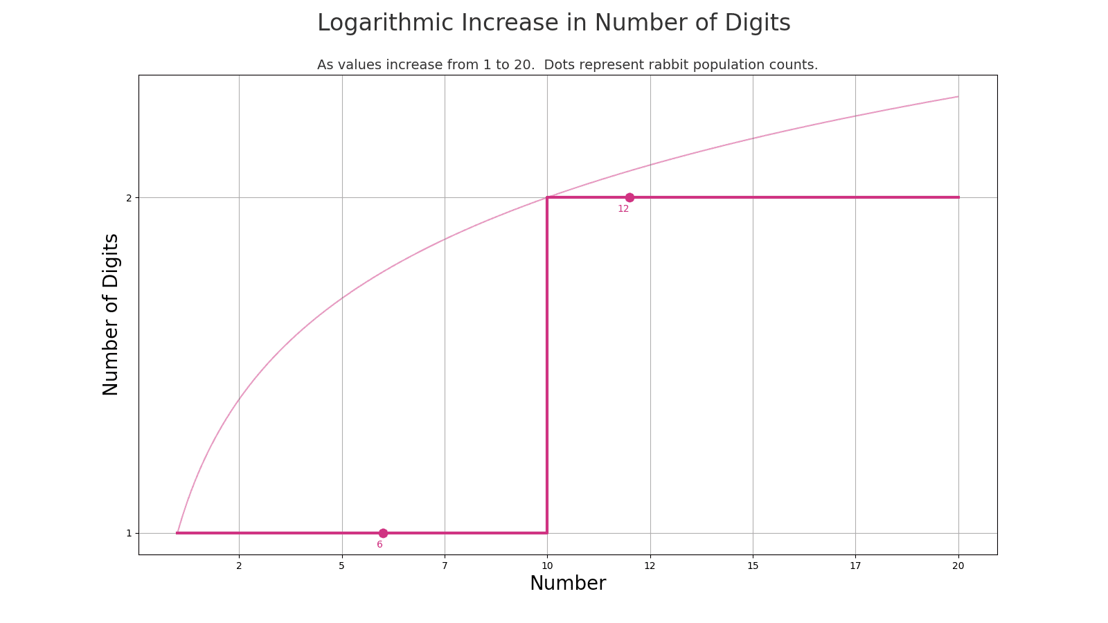
By Generation 2, we've reached 12 rabbits, now a two-digit number. This chart shows the number rising in value:
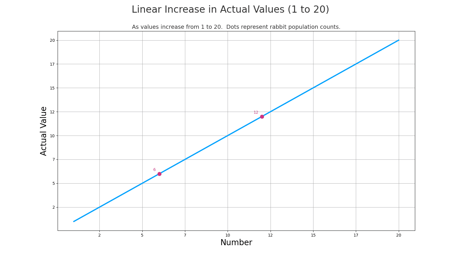
As we cross into the next order of magnitude, the bucket of numbers that start with "1" is as big as the bucket of all the numbers that came before it. If you were jogging along at a steady pace, then you would be cranking up in lead digits as you went from 7 to 8 to 9, but then you would be stuck in the 10s for as long as it took you to get here.
In terms of lead digits, the left side of this chart increases linearly: 1, 2, 3, 4, 5, 6...
But the right side of the chart is all "1" for a lead digit. It doesn't change.
If you were counting up one by one then you would cover all of the lead digits. But rabbits don't breed at a steady pace, they breed at an exponential rate. Their population size jumps up at a rate that mirrors the logarithmic increase in the number of digits of the population count number.
By Generation 6, the population hits 192, marking our first transition to a three-digit number. We skipped a lot of lead digits in the two-digit numbers, but yet again, we're stuck in the low-lead-digit numbers since there are as many three-digit numbers starting with "1" as there were numbers before us. When we cross to this next order of magnitude, we're still at the lower end of it. Since the bucket of three-digit numbers that starts with "1" is as big as the bucket of all the numbers that came before it.
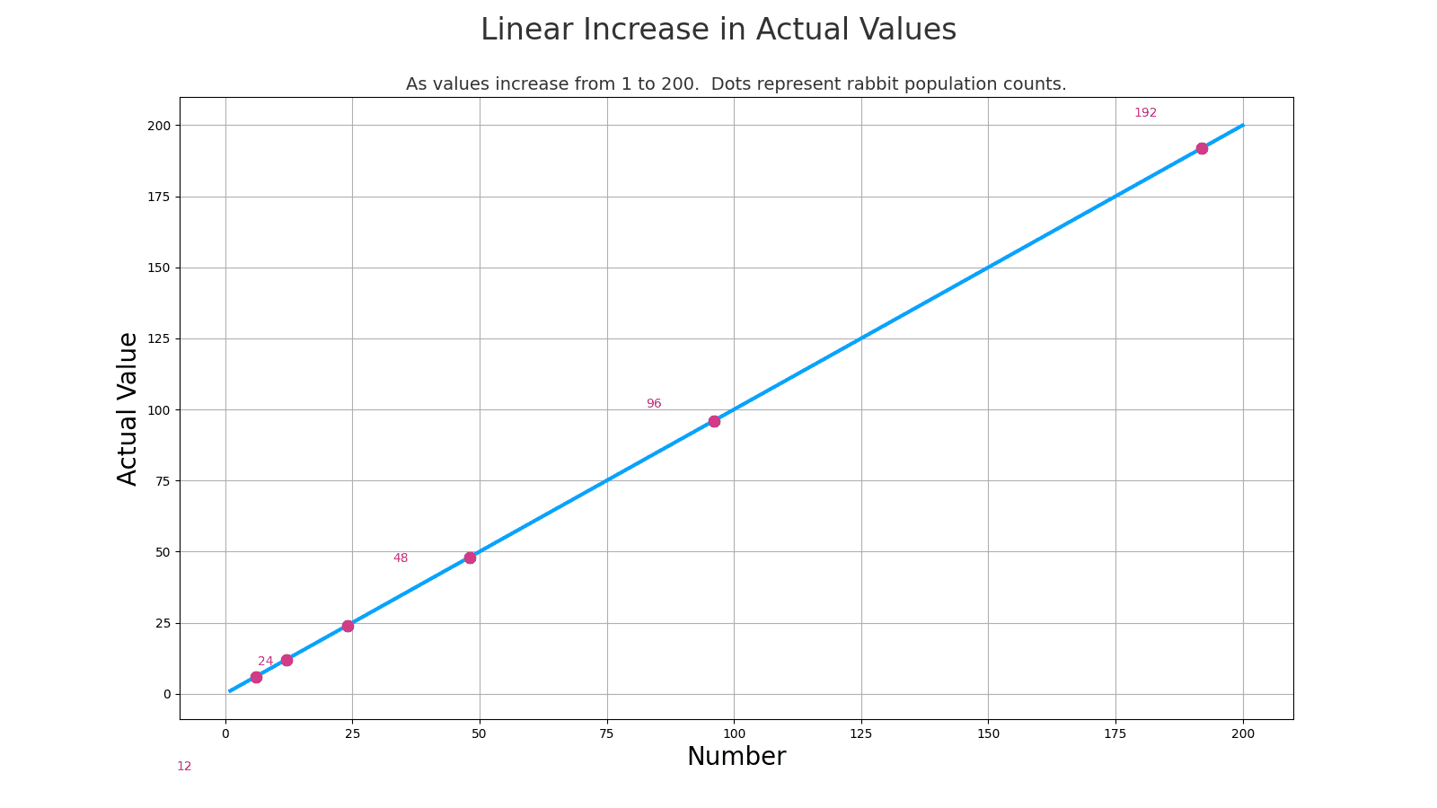
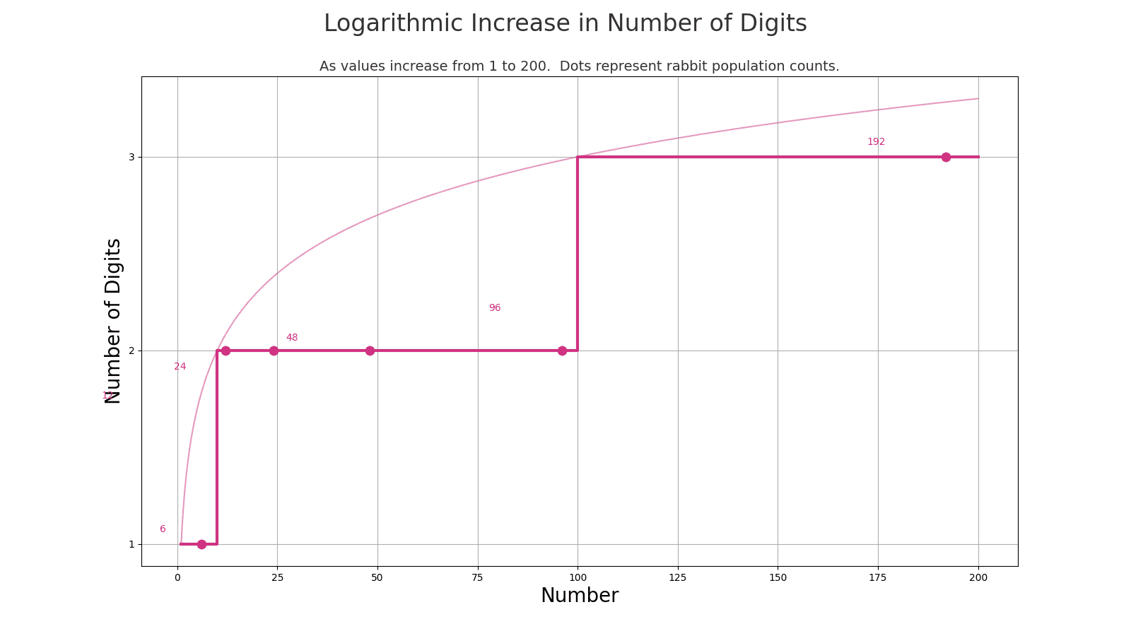
Let's take a look at the relationship between the population value and the number of digits in the population count, all the way up to 2,000, a four-digit number:
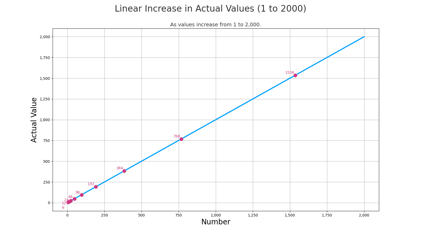
The chart shows the numbers increasing linearly: 1, 2, 3, 4, 5, etc. That's the blue line. The dots represent the rabbit population counts at each generation: 6, 12, 48, 96, 192...
Notice how the dots are packed together on the left side but then they spread out. They don't follow the linear increase of simply counting up from 1. The rabbit population counts increase in a different way: Each new number depends on the previous number. That's the special factor that has to be present for Benford's Law to apply.
Now, instead of looking at the actual values of the numbers as we count up from 1 to 2,000, let's look at the number of digits in the number. At first, you're at one-digit numbers. At 10, you have hit two-digit numbers. That digit count is the Y axis on this chart, going up to 4 for 2,000, which is a four-digit number.
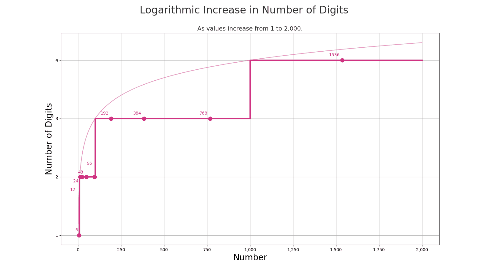
See the point where the rabbit population goes from 768 to 1,536? That's an order-of magnitude jump in population, meaning that the population count has gained a digit. But look at what happens to the lead digit when that happens: From 100 to 1000, the lead digit was going up and up. But there's as much space on the right side of that chart, above 1000, where the lead digit is a "1" as in the entire left side of the chart, when the lead digit was increasing. Suddenly, the lead digit is thrown back down to the low digits. And because everything is at a greater scale now at this new four-digit magnitude, there's a lot more horizontal space between lead digit changes now.
That's the essence of Benford's Law: Exponential growth patterns increase in a way that tracks the way that the number of digits increases. Types of growth that don't build on the previous value don't. Natural processes like investments and rabbit populations grow in ways that depend on the previous value.
Another interesting thing about Benford's Law: You don't really have to understand why it happens to understand how to use it. So, don't worry too much if you didn't follow the math.
Conclusion
Benford's Law, with its unique insight into aggregate data, already plays a role in various applications, from fraud detection to financial analysis. However, its potential extends further, particularly in shaping the future of AI.
One intriguing application lies in crafting datasets for training AI models. By ensuring these datasets adhere to Benford's Law, we could enhance the realism and reliability of the training process, leading to more robust and accurate AI models. Benford's Law could be used in areas like evaluation metrics in AI, offering a novel lens to assess the authenticity and accuracy of AI-generated data.
While its current applications are well-established, the future might see Benford's Law becoming a part of the AI toolkit, guiding both the development and evaluation of AI models in various fields. This exploration could pave the way for AI systems that resonate more deeply with the patterns found in natural data.
Lab
Don't take my word for it. You can reproduce all of my findings and visuals from this article with Python notebooks on Google Collab, in this GitHub repository.

Data.gov datasets
You can download datasets from Data.gov to Collab and do your own lead-digit analysis with this notebook: Benford's Law Demo, or see it on GitHub.
Play with it: Find your own datasets and try it. Find any dataset that you think might work and copy the CSV download link to the notebook. Download the file yourself ahd look at it to find the column name of the column that you think might demonstrate a distribution that follows the prediction from Benford's Law.
Money laundering simulation
You can use the notebook for the structured-transaction simulation to reproduce my findings. Run the simulation a few times and look at the different values that you get for the three different measures of how the actual distribution varies from the Benford's Law predicted distribution for the two different scenarios. Random numbers are random: The statistics won't always magically detect every money launderer. Sometimes they'll even go backwards. Random!
Then, change the parameters. Instead of a thousand transactions per day, lower it to 100. Lower the percentage of structured transactions. How low can you go before the differing lead-digit distributions are imperceptible in terms of how they correspond with the Benford's Law predictions? If you increase the number of structured transactions then does it enhance the distinction?